Lambert W function and exponent of Lambert W function
for C99
Nov. 7 2020
Takayuki HOSODA


 Japanese edition is here.
The Lambert W function is also known as the omega function or product logarithm, named after Johann Heinrich Lambert in France (26 or 28 August 1728-25 September 1777). It is a multi-valued function and is a branch of the inverse function of the function f (wj= w e w. Where w is any complex number and e w is an exponential function. A principal branch with a Lambert W function value greater than or equal to -1 is represented as W 0.
eW0 — Exponent of the principal branch of the Lambert W functionCalculation example of cexplambertw()eW0(x) — the exponent of the principal branch of the Lambert W function W0(x) — can be calculated by using Newton-Raphson method,
or Halley's method shown below.

When finding eW using an iterative method such as Newton's Rapson method, giving a bad initial value, especially when it is very close to the singularity x = -1 / e, can be terrible in terms of convergence. Therefore, it is desirable that the initial value asymptotically approaches eW at the singularity. For that reason, I chose the following formula as an approximate expression that gives the initial value. This equation replaces the coefficient 1/3 of the third term of the Puiseux series expansion near x = -1 / e of e W0 with 0.3 and ignores the fourth and subsequent terms.
Initial approximation :
Series expansion of eW at z = -1 / e (Puiseux series) :
Instead of the coefficient of 0.3 in the formula above, it can be (e - √2 - 1) which make it zero at x = 0,
or "1 / 3" from Puiseux series, but 0.3 is quite good enough for this purpose.
From the relation below, the Lambert W can be calculated by using eW — the exponent of Lambert W function.

cexplambertw.c (C99) NAME cexplambertw -- exponent of the principal branch of the complex Lambert W function. LIBRARY Math library (libm, -lm) SYNOPSIS #include <math.h> #include <complex.h> double complex cexplambertw(complex double x); RETURN VALUE cexplambertw(x) returns requested exponent of the principal branch of the complex Lambert W function.Recurrence formula (Halleys method) :Initial approximation :

/* cexplambertw : exponent of Lambert W0 function
    Rev.1.52 (Dec. 4, 2020) (c) Takayuki HOSODA (aka Lyuka)
    http://www.finetune.co.jp/~lyuka/technote/lambertw/
    Acknowledgments: Thanks to Albert Chan for his informative suggestions.
 */
#include <math.h>
#include <complex.h>

#ifdef HAVE_NO_CLOG
double complex clog(double complex);
double complex clog(double complex x) {
    return log(cabs(x)) + atan2(cimag(x), creal(x)) * I;
}
#endif

double complex cexplambertw(double complex);
double complex cexplambertw(double complex x) {
    double complex y, p, s, t;
    double q, r, m;

    r = 1 / M_E;
    q = M_E - M_SQRT2 - 1;
    if ((fabs(creal(x)) <= (DBL_MAX / 1024.0)) && (fabs(cimag(x)) <= (DBL_MAX / 1024.0))) {
        m = 1.0;
        s = x + r;
        if (s == 0) return r;
        y = (r + csqrt((2.0 * r) * s) + q * s); // approximation near x=-1/e
    } else {
        m = (1.0 / 1024.0);
        x *= m; // scaling
        s = x * m;
        y = r * m + csqrt(r * (s * 64.0)) + q * s;
        y *= 1024.0;
    }
    r = DBL_MAX;
    do {
        q = r; p = y;
        t = clog(y);
        s =  0.5 * (x / y - t * m) / (1 + t) + (1 + t) * m;
        t = (x - y * (t * m));
        y += t / s;
        r = cabs(y - p); // correction radius
    } while (r != 0 && q > r);// convergence check by Urabe's theorem
    return p;
}
W0 — The principal branch of the Lambert W functioncexplambertw(1 - i2) = 1.963022024795711 - i1.157904818620495 (i2.220446049250313e-16) cexplambertw(1) = 1.763222834351897 cexplambertw(i) = 1.219531415904638 + i0.7927604805362661 cexplambertw(0) = 1 cexplambertw(-0.36) = 0.4466034047150879 (5.551115123125783e-17) cexplambertw(-0.3678794411714423) = 0.3678794411714423 cexplambertw(-0.37) = 0.3671727690033079 + i0.03950593783033725 (0 - i1.52655665885959e-16) cexplambertw(-1) = 0.168376379087223 + i0.7077541887847276 (-5.551115123125783e-17 + i0) cexplambertw(-1.78) = -0.05991375474182515 + i1.091676160700024 (2.081668171172169e-17 + i0) cexplambertw(-6 + i8) = 0.5264016089780164 + i4.672167782982316 (-1.110223024625157e-16 + i0) cexplambertw(-1e+40 + i1e+40) = -1.105839096727962e+38 + i1.166002733393464e+38 cexplambertw(1e+99) = 4.493356750426822e+96 cexplambertw(1.797693134862316e+308 + i0) = 2.556348163871691e+305 + i0 (-3.89812560456e+289 + i0) cexplambertw(-1.797693134862316e+308 + i0) = -2.556297327179282e+305 + i1.140377281032545e+303 cexplambertw(1.797693134862316e+308 + i1.797693134862316e+308) = 2.557935739687931e+305 + i2.552239351260207e+305 cexplambertw(-1.797693134862316e+308 + i1.797693134862316e+308) = -2.546517666521172e+305 + i2.563606662249022e+305 (3.89812560456e+289 + i0) cexplambertw(0 + i1.797693134862316e+308) = 5.701971348523801e+302 + i2.556335454509411e+305 (7.613526571406249e+286 + i0)
Calculation example of clambertw()It is necessary to consider the singularity, but since eW does not become zero, it was relatively easy to find eW by Newton-Raphson method or Harrey's method. However, when trying to find W0 - Lambert's W of the primary branch by such an iterative method, since W0 becomes zero when x is zero, so it is necessary to consider zero as well as the singularity. In other words, it is strongly desired that the approximation formula of the initial value of the iterative method has an asymptotic to zero error at the singular point and zero. Also, since W0 is, from the singularity, a monotonically increasing function, its approximation must also be a monotonically increasing function. To meet these requirements, the initial value is calculated using the following approximation function.

Since W0 has a large derivative around the singularity, Newton's method can cause catastrophic behavior near the singularity if the initial approximation is poor or due to computational errors. Therefore, we will use the Halley method or Householder's method of order 4, which is more stable than the Newton method, to obtain W0.
Newton-Raphson method :
Halley's method :
Householder's method of order 4 :

clambertw.c (C99) NAME clambertw -- the principal branch of the complex Lambert W function. LIBRARY Math library (libm, -lm) SYNOPSIS #include <math.h> #include <complex.h> double complex clambertw(complex double x); RETURN VALUE clambertw(x) returns complex value of the principal branch of the Lambert W function.Recurrence formula (Halley's method) :Initial approximation :
/* clambertw : Lambert W0 function
    Rev.1.52 (Dec. 4, 2020) (c) Takayuki HOSODA (aka Lyuka)
    http://www.finetune.co.jp/~lyuka/technote/lambertw/
    Acknowledgments: Thanks to Albert Chan for his informative suggestions.
 */
#include <math.h>
#include <complex.h>
#include <float.h>

#ifdef HAVE_NO_CLOG
double complex clog(double complex);
double complex clog(double complex x) {
    return log(cabs(x)) + atan2(cimag(x), creal(x)) * I;
}
#endif

double complex clambertw(double complex);
double complex clambertw(double complex x) {
    double complex y, p, s, t;
    double q, r, m;

    r = 1 / M_E;
    q = M_E - M_SQRT2 - 1;
    if ((fabs(creal(x)) <= (DBL_MAX / 1024.0)) && (fabs(cimag(x)) <= (DBL_MAX / 1024.0))) {
        m = 1.0;
        s = x + r;
        if (s == 0) return -1;
        y = clog(r + csqrt((2.0 * r) * s) + q * s); // approximation near x=-1/e
    } else {
        m = (1.0 / 1024.0);
        x *= m; // scaling
        s = x * m;
        y = clog(r * m + csqrt(r * (s * 64.0)) + q * s);
        y += (M_LN2 * 10.0);
    }
    r = DBL_MAX;
    do {
        q = r; p = y;
        t = cexp(y) * m;
        s = y * t - x;
        u = (0.5 * y) / (y + 1.0) * s + t + x;
        y -= s / u;// Halley's method
        r = cabs(y - p); // correction radius
    } while (r != 0 && q > r); // convergence check by Urabe's theorem
    return p;
}
Calculation results by WolframAlphaclambertw(2.718281828459045 + i0) = 0.9999999999999999 + i0 (1.110223024625157e-16 + i0) clambertw(1 - i2) = 0.8237712167092305 - i0.5329289867954415 (0 - i1.110223024625157e-16) clambertw(1 + i0) = 0.5671432904097838 + i0 clambertw(0 + i1) = 0.3746990207371175 + i0.5764127230314353 (-5.551115123125783e-17 + i0) clambertw(0 + i0) = 0 + i0 clambertw(-0.36 + i0) = -0.8060843159708175 + i0 (-2.220446049250313e-16 + i0) clambertw(-0.3678794411714423 + i0) = -1 + i0 clambertw(-0.37 + i0) = -0.996167692712445 + i0.1071826188083488 (3.33066907387547e-16 + i1.956768080901838e-15) clambertw(-1 + i0) = -0.3181315052047642 + i1.337235701430689 (1.110223024625157e-16 + i2.220446049250313e-16) clambertw(-1.78 + i0) = 0.08921804985620939 + i1.625623674427768 (-6.938893903907228e-17 + i0) clambertw(-6 + i8) = 1.547930197079636 + i1.458601930168348 clambertw(-1e+40 + i1e+40) = 87.9726013585729 + i2.329718360883123 clambertw(1e+99 + i0) = 222.5507689557502 + i0 clambertw(1.797693134862316e+308 + i0) = 703.2270331047702 + i0 clambertw(-1.797693134862316e+308 + i0) = 703.2270231685106 + i3.137131632158036 clambertw(0 + i1.797693134862316e+308) = 703.2270306206868 + i1.568565805021136 clambertw(-1.797693134862316e+308 + i1.797693134862316e+308) = 703.5731090989279 + i2.352850357853284 clambertw(1.797693134862316e+308 + i1.797693134862316e+308) = 703.5731140622003 + i0.7842834489371958
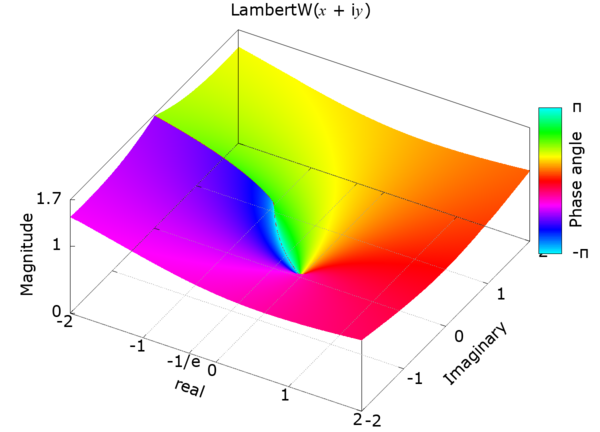
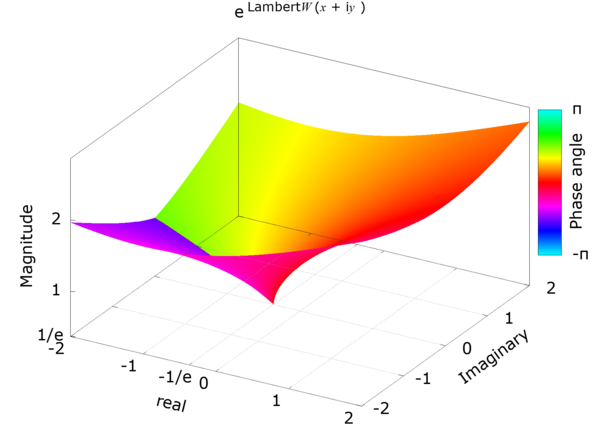
4D plot of complex LambertW using gnuplot splot with pm3d -- Plot scripts, data and reference images.Reference
Download : lambertw-gnuplot-pm3d.zip [5MB zip]

![[Mail]](/~lyuka/images/mail.gif)


 © 2000 Takayuki HOSODA.